How To Draw A Density Curve
How To Draw A Density Curve - Therefore, the last answer is a common sense. Hence the total area under the density curve will always be equal to 1. A density curve lets us visually see where the mean and the median of a distribution are located. Web we are breaking out the density plot into multiple density plots based on species. This area property of the density curve plays a crucial role in statistics and machine learning. Web learn about the importance of density curves and their properties. Now estimate the inflection points as shown below: Web the density curve covers all possible data values and their corresponding probabilities. You can also add a line for the mean using the function geom_vline. To fit both on the same graph, one or other needs to be rescaled so that their areas match.
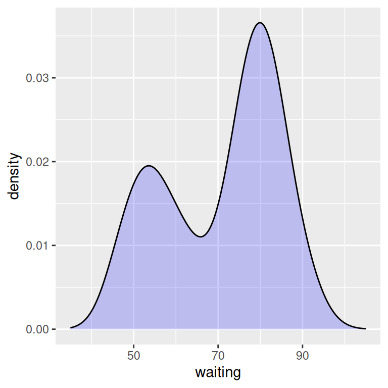
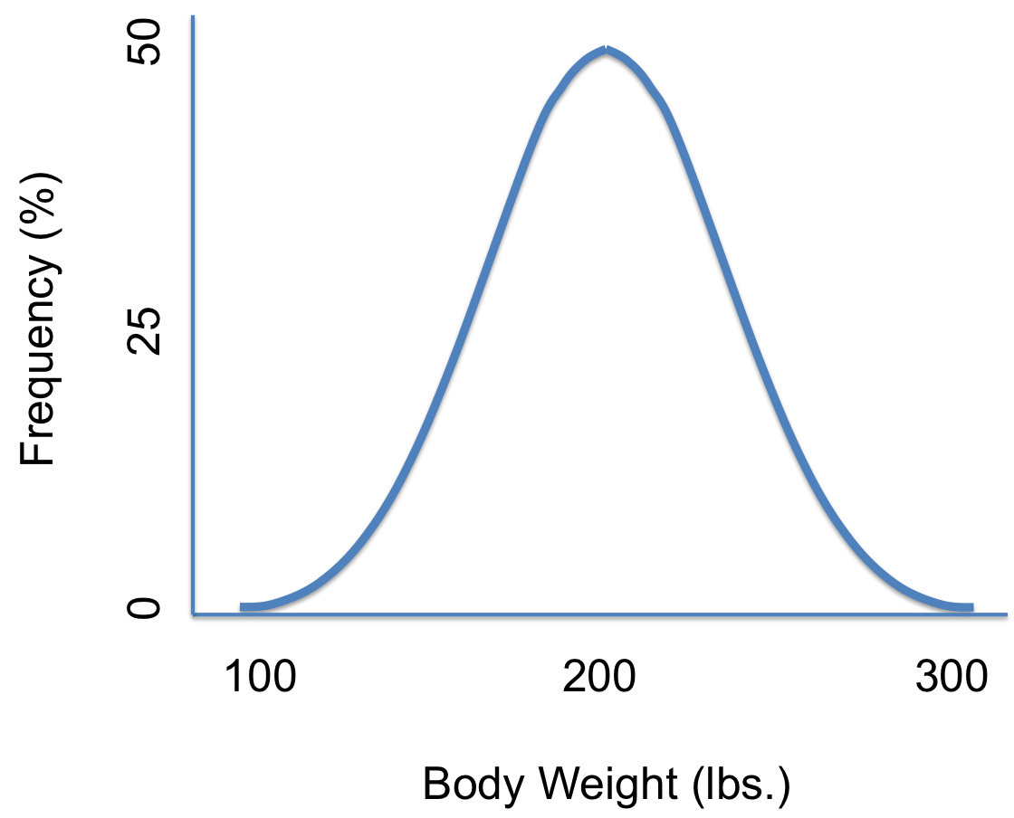
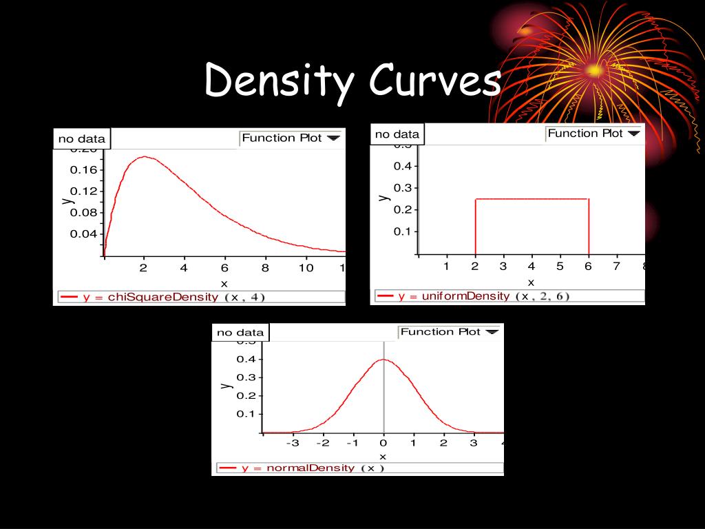
A density curve lets us visually see where the mean and the median of a distribution are located. The median is located at the center of the data. A density curve gives us a good idea of the “shape” of a distribution, including whether or not a distribution has one or more “peaks” of frequently occurring values and whether or not the distribution is skewed to the left or the right. The total area under the curve results probability value of 1. Web this r tutorial describes how to create a density plot using r software and ggplot2 package. Density curves with adjust set to.25 (red), default value of 1 (black), and 2 (blue) in this example, the x range is automatically set so that it contains the data, but this. Web to create a normal distribution plot with mean = 0 and standard deviation = 1, we can use the following code: Web the area under a density curve equals 1, and the area under the histogram equals the width of the bars times the sum of their height ie. Web we are breaking out the density plot into multiple density plots based on species. We’ll explore it further in the next post.
Density plot with multiple airlines. This would lead to an estimate of about 0.05 for the standard. The median is located at the center of the data. Web to create a normal distribution plot with mean = 0 and standard deviation = 1, we can use the following code: Hence the total area under the density curve will always be equal to 1. Web the mean is greater than the median, and the curve appears to have a longer right tail.left skewed (negative skew): Web histogram with density line. To fit both on the same graph, one or other needs to be rescaled so that their areas match. A density curve lets us visually see where the mean and the median of a distribution are located. A basic histogram can be created with the hist function.

Solved 1. Sketch density curves that describe distributions
And we draw like this. This is a normal distribution curve representing probability density function. The area under the curve corresponds to the cumulative relative frequencies, which should sum up to 100% or 1. Web probabilities from density curves. If we add more bars to the graph, like in the example histogram below, we get something that’s starting to look.

How to make a density graph
Web the area of a rectangle is height x width, so if you multiply the height x width in this case you would get.5 x 1 =.5. The median is located at the center of the data. One density plot curve for each value of the categorical variable, species. 5 or 10 is usually a disaster. I was confused at.
6.3 Making a Density Curve R Graphics Cookbook, 2nd edition
The total area under the curve results probability value of 1. If you add up all of the areas of these rectangles. Add them together and you get.5 +.5 =1. 5 or 10 is usually a disaster. Web we are breaking out the density plot into multiple density plots based on species.

AP Stats Density Curve Basics YouTube
The median is located at the center of the data. Probability in normal density curves. The mean and median are the same for a symmetric density curve. Web courses on khan academy are always 100% free. Figure 6.9 shows what happens with a smaller and larger value of adjust:
Density Curve Examples Statistics How To
Start practicing—and saving your progress—now: Using frequency scale is possible, but requires more work than above. In a left skewed distribution, the mean is on the left closer to the tail of the distribution. Web learn about the importance of density curves and their properties. Web sal said the area underneath any density curve is going to be 1.

What are Density Curves? (Explanation & Examples) Statology
We’ll explore it further in the next post. In a left skewed distribution, the mean is on the left closer to the tail of the distribution. Hence the total area under the density curve will always be equal to 1. Web this distribution is fairly normal, so we could draw a density curve to approximate it as follows: The area.

What are Density Curves? (Explanation & Examples) Statology
If you add up all of the areas of these rectangles. Web overlapping histograms can be complicated enough with say 2 groups: Using frequency scale is possible, but requires more work than above. Web we are breaking out the density plot into multiple density plots based on species. Web sal said the area underneath any density curve is going to.

Tutorial 9 Density 2d Plot Data Visualization Using R vrogue.co
A density curve gives us a good idea of the “shape” of a distribution, including whether or not a distribution has one or more “peaks” of frequently occurring values and whether or not the distribution is skewed to the left or the right. Web the mean is greater than the median, and the curve appears to have a longer right.
PPT Density Curves and the Normal Distribution PowerPoint
Density curves with adjust set to.25 (red), default value of 1 (black), and 2 (blue) in this example, the x range is automatically set so that it contains the data, but this. Web the bandwidth can be set with the adjust parameter, which has a default value of 1. Web to create a normal distribution plot with mean = 0.
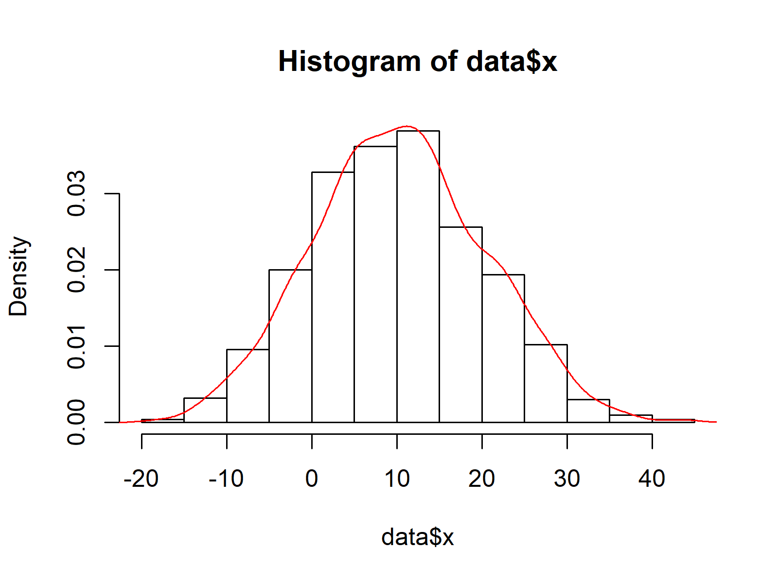
Overlay Histogram with Fitted Density Curve Base R & ggplot2 Example
Small multiple version of an ggplot density plot Start practicing—and saving your progress—now: If you add up all of the areas of these rectangles. Web the bandwidth can be set with the adjust parameter, which has a default value of 1. Density curves with adjust set to.25 (red), default value of 1 (black), and 2 (blue) in this example, the.
The Total Area Under The Curve Results Probability Value Of 1.
If we add more bars to the graph, like in the example histogram below, we get something that’s starting to look like a curve. Web density values can be greater than 1. Density curves with adjust set to.25 (red), default value of 1 (black), and 2 (blue) in this example, the x range is automatically set so that it contains the data, but this. Web probabilities from density curves.
And We Draw Like This.
If you add up all of the areas of these rectangles. In a right skewed distribution, the mean is on the right closer to. Figure 6.9 shows what happens with a smaller and larger value of adjust: The mean is less than the median, and the curve appears to have a longer left tail.
Web The Density Curve Covers All Possible Data Values And Their Corresponding Probabilities.
Add them together and you get.5 +.5 =1. Web this distribution is fairly normal, so we could draw a density curve to approximate it as follows: Math > statistics and probability > random variables >. Web the area under a density curve equals 1, and the area under the histogram equals the width of the bars times the sum of their height ie.
Web Courses On Khan Academy Are Always 100% Free.
Web the mean is greater than the median, and the curve appears to have a longer right tail.left skewed (negative skew): Now estimate the inflection points as shown below: Therefore, the last answer is a common sense. A density curve gives us a good idea of the “shape” of a distribution, including whether or not a distribution has one or more “peaks” of frequently occurring values and whether or not the distribution is skewed to the left or the right.